Develidağ TAS¶

import numpy as np
import pandas as pd
import matplotlib.pyplot as plt

dataset = pd.read_excel("./D2004_1.xlsx", index_col=0)
dataset

dataset.loc['Na2O+K2O']

D2004-1     5.155620
D2004-3     4.776985
D2004-4     5.220545
D2004-5     5.586280
D2004-7     4.934305
D2004-8     4.817385
D2004-10    4.293880
D2004-11    4.277170
D2004-12    4.651450
D2004-13    6.040070
Name: Na2O+K2O, dtype: float64

coords = np.array([(41, 3), (45, 3), (45, 5), (52, 5), (41, 7), (49.4, 7.3), (45, 9.4), (48.4, 11.5), (52.5, 14),
                   (53, 9.3), (57.6, 11.7), (61, 13.5), (57, 5.9), (63, 7), (69, 8)])

plt.figure(figsize=(10.5, 9))
plt.scatter(coords[:, 0], coords[:, 1], color="black")

plt.plot((45, 52), (5, 5), "k-")
plt.plot((41, 45), (3, 3), "k-")
plt.plot((45, 61), (5, 13.5), "k-")
plt.plot((45, 52.5), (9.4, 14), "k-")
plt.plot((41, 45), (7, 9.4), "k--")
plt.plot((41, 41), (3, 7), "k--")
plt.plot((41, 41), (1, 3), "k-")
plt.plot((52, 69), (5, 8), "k-")
plt.plot((45, 45), (1, 5), "k-")
plt.plot((52, 52), (1, 5), "k-")
plt.plot((52, 49.4), (5, 7.3), "k-")
plt.plot((49.4, 45), (7.3, 9.4), "k-")
plt.plot((57, 57), (5.9, 1), "k-")
plt.plot((63, 63), (7, 1), "k-")
plt.plot((57, 53), (5.9, 9.3), "k-")
plt.plot((53, 48.4), (9.3, 11.5), "k-")
plt.plot((63, 57.6), (7, 11.7), "k-")
plt.plot((57.6, 52.5), (11.7, 14), "k-")
plt.plot((69, 69), (8, 13), "k-")
plt.plot((69, 76), (8, 1), "k-")

plt.text(66, 4, "Dacite", fontsize=16, weight="bold")
plt.text(60, 4, "Andesite", fontsize=16, weight="bold", ha="center")
plt.text(54.5, 3.8, "Basaltic\n Andesite", fontsize=12, weight="bold", ha="center")
plt.text(48.5, 4, "Basalt", fontsize=16, weight="bold", ha="center")
plt.text(43, 1.5, "Picro-\n Basalt", fontsize=14, weight="bold", ha="center")
plt.text(48.8, 5.2, "Trachy-\n Basalt", fontsize=12, weight="bold", ha="center")
plt.text(53, 5.9, "Basaltic\n trachyandesite", fontsize=12, weight="bold", ha="center", rotation=-30)
plt.text(58, 7.5, "Trachyandesite", fontsize=14, weight="bold", ha="center", rotation=-25)
plt.text(44, 12, "Foidite", fontsize=16, weight="bold", ha="center")
plt.text(48.9, 9.35, "Phonotephrite", fontsize=12, weight="bold", ha="center")
plt.text(53, 11.5, "Tephriphonolite", fontsize=13, weight="bold", ha="center")
plt.text(57, 13.5, "Phonolite", fontsize=14, weight="bold", ha="center")
plt.text(64.5, 11, "Trachyte\n (Q < 20%)", fontsize=14, weight="bold", ha="center")
plt.text(64.5, 9.5, "Trachydacite\n (Q > 20%)", fontsize=14, weight="bold", ha="center")
plt.text(45.2, 7.5, "Tephrite\n (O < 10%)", fontsize=12, weight="bold", ha="center")
plt.text(44, 6, "Basanite\n (O > 10%)", fontsize=12, weight="bold", ha="center")

plt.xlabel(r'$SiO_{2} \ (wt \ \%)$'), plt.ylabel(r'$Na_{2}O \ \plus  K_{2}O \ (wt \ \%)$')
plt.title("TAS")
plt.show()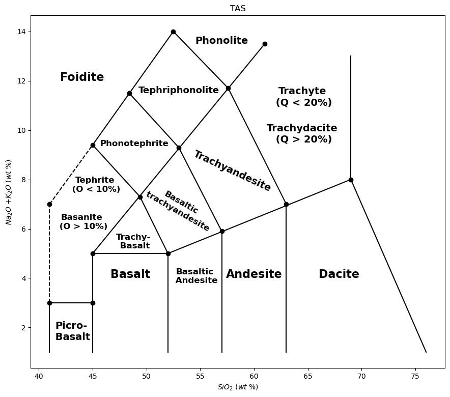

coords = np.array([(41, 3), (45, 3), (45, 5), (52, 5), (41, 7), (49.4, 7.3), (45, 9.4), (48.4, 11.5), (52.5, 14),
                   (53, 9.3), (57.6, 11.7), (61, 13.5), (57, 5.9), (63, 7), (69, 8)])

plt.figure(figsize=(11.5, 10))
#plt.scatter(coords[:, 0], coords[:, 1], color="black")

plt.plot((45, 52), (5, 5), "k-")
plt.plot((41, 45), (3, 3), "k-")
plt.plot((45, 61), (5, 13.5), "k-")
plt.plot((45, 52.5), (9.4, 14), "k-")
plt.plot((41, 45), (7, 9.4), "k--")
plt.plot((41, 41), (3, 7), "k--")
plt.plot((41, 41), (1, 3), "k-")
plt.plot((52, 69), (5, 8), "k-")
plt.plot((45, 45), (1, 5), "k-")
plt.plot((52, 52), (1, 5), "k-")
plt.plot((52, 49.4), (5, 7.3), "k-")
plt.plot((49.4, 45), (7.3, 9.4), "k-")
plt.plot((57, 57), (5.9, 1), "k-")
plt.plot((63, 63), (7, 1), "k-")
plt.plot((57, 53), (5.9, 9.3), "k-")
plt.plot((53, 48.4), (9.3, 11.5), "k-")
plt.plot((63, 57.6), (7, 11.7), "k-")
plt.plot((57.6, 52.5), (11.7, 14), "k-")
plt.plot((69, 69), (8, 13), "k-")
plt.plot((69, 76), (8, 1), "k-")

plt.text(66, 4, "Dacite", fontsize=16, weight="bold", alpha=0.3)
plt.text(60, 4, "Andesite", fontsize=16, weight="bold", ha="center", alpha=0.3)
plt.text(54.5, 3.8, "Basaltic\n Andesite", fontsize=12, weight="bold", ha="center", alpha=0.3)
plt.text(48.5, 4, "Basalt", fontsize=16, weight="bold", ha="center", alpha=0.3)
plt.text(43, 1.5, "Picro-\n Basalt", fontsize=14, weight="bold", ha="center", alpha=0.3)
plt.text(48.8, 5.2, "Trachy-\n Basalt", fontsize=12, weight="bold", ha="center", alpha=0.3)
plt.text(53, 5.9, "Basaltic\n trachyandesite", fontsize=12, weight="bold", ha="center", rotation=-30, alpha=0.3)
plt.text(58, 7.5, "Trachyandesite", fontsize=14, weight="bold", ha="center", rotation=-25, alpha=0.3)
plt.text(44, 12, "Foidite", fontsize=16, weight="bold", ha="center", alpha=0.3)
plt.text(48.9, 9.35, "Phonotephrite", fontsize=12, weight="bold", ha="center", alpha=0.3)
plt.text(53, 11.5, "Tephriphonolite", fontsize=13, weight="bold", ha="center", alpha=0.3)
plt.text(57, 13.5, "Phonolite", fontsize=14, weight="bold", ha="center", alpha=0.3)
plt.text(64.5, 11, "Trachyte\n (Q < 20%)", fontsize=14, weight="bold", ha="center", alpha=0.3)
plt.text(64.5, 9.5, "Trachydacite\n (Q > 20%)", fontsize=14, weight="bold", ha="center", alpha=0.3)
plt.text(45.2, 7.5, "Tephrite\n (O < 10%)", fontsize=12, weight="bold", ha="center", alpha=0.3)
plt.text(44, 6, "Basanite\n (O > 10%)", fontsize=12, weight="bold", ha="center", alpha=0.3)

xx = np.linspace(45, 65, 1000)
p = np.polyfit(dataset.loc['SiO2'], dataset.loc['Na2O+K2O'], 2)
f = np.poly1d(p)
plt.plot(xx, f(xx), "g-", lw=2)


plt.plot(dataset.loc['SiO2'], dataset.loc['Na2O+K2O'], "o", markersize=8.5)

# Add labels for each point (extract numbers from index like 'D2004-1' → '1')
for idx in dataset.columns:  # Assuming columns are 'D2004-1', 'D2004-2', etc.
    if idx.startswith("D2004-"):  # Check if index follows the expected format
        number = idx.split("-")[-1]  # Extract the part after 'D2004-'
        x = dataset.loc['SiO2', idx]  # X-coordinate (SiO2 value)
        y = dataset.loc['Na2O+K2O', idx]  # Y-coordinate (Na2O+K2O value)
        plt.text(x, y, number, ha='center', va='center', fontsize=7)  # Label above point

plt.xlabel(r'$SiO_{2} \ (wt \ \%)$'), plt.ylabel(r'$Na_{2}O \ \plus  K_{2}O \ (wt \ \%)$')
plt.title("TAS")
plt.show()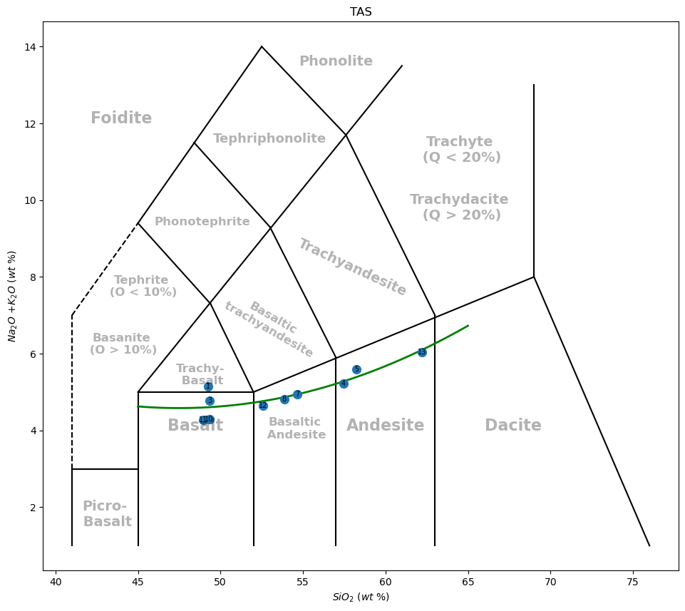

import matplotlib.pyplot as plt

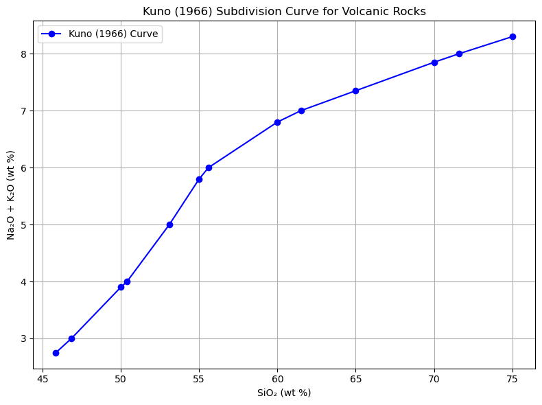
# Kuno (1966) coordinates: (SiO2, Na2O + K2O)
kuno_coords = [
    (45.85, 2.75), (46.85, 3.0), (50.0, 3.9), (50.4, 4.0),
    (53.1, 5.0), (55.0, 5.8), (55.6, 6.0), (60.0, 6.8),
    (61.5, 7.0), (65.0, 7.35), (70.0, 7.85), (71.6, 8.0),
    (75.0, 8.3)
]

# Split into two lists
x_vals, y_vals = zip(*kuno_coords)

# Plotting
plt.figure(figsize=(8, 6))
plt.plot(x_vals, y_vals, marker='o', linestyle='-', color='blue', label='Kuno (1966) Curve')
plt.xlabel('SiO₂ (wt %)')
plt.ylabel('Na₂O + K₂O (wt %)')
plt.title('Kuno (1966) Subdivision Curve for Volcanic Rocks')
plt.grid(True)
plt.legend()
plt.tight_layout()
plt.show()

zoom

coords = np.array([(41, 3), (45, 3), (45, 5), (52, 5), (41, 7), (49.4, 7.3), (45, 9.4), (48.4, 11.5), (52.5, 14),
                   (53, 9.3), (57.6, 11.7), (61, 13.5), (57, 5.9), (63, 7), (69, 8)])

# Kuno (1966) coordinates: (SiO2, Na2O + K2O)
kuno_coords = [
    (45.85, 2.75), (46.85, 3.0), (50.0, 3.9), (50.3, 4.0),
    (53.1, 5.0), (55.0, 5.8), (55.6, 6.0), (60.0, 6.8),
    (61.5, 7.0), (65.0, 7.35), (70.0, 7.85), (71.6, 8.0),
    (75.0, 8.3), (76.4, 8.4)
]
# Split into two lists
x_vals, y_vals = zip(*kuno_coords)

plt.figure(figsize=(11.5, 10))
#plt.scatter(coords[:, 0], coords[:, 1], color="black")
plt.plot(x_vals, y_vals, marker='o', markersize=5, linestyle='-', color='black', label='Kuno (1966) Curve')

plt.plot((45, 52), (5, 5), "k-")
plt.plot((41, 45), (3, 3), "k-")
plt.plot((45, 61), (5, 13.5), "k-")
plt.plot((45, 52.5), (9.4, 14), "k-")
plt.plot((41, 45), (7, 9.4), "k--")
plt.plot((41, 41), (3, 7), "k--")
plt.plot((41, 41), (1, 3), "k-")
plt.plot((52, 69), (5, 8), "k-")
plt.plot((45, 45), (1, 5), "k-")
plt.plot((52, 52), (1, 5), "k-")
plt.plot((52, 49.4), (5, 7.3), "k-")
plt.plot((49.4, 45), (7.3, 9.4), "k-")
plt.plot((57, 57), (5.9, 1), "k-")
plt.plot((63, 63), (7, 1), "k-")
plt.plot((57, 53), (5.9, 9.3), "k-")
plt.plot((53, 48.4), (9.3, 11.5), "k-")
plt.plot((63, 57.6), (7, 11.7), "k-")
plt.plot((57.6, 52.5), (11.7, 14), "k-")
plt.plot((69, 69), (8, 13), "k-")
plt.plot((69, 76), (8, 1), "k-")

plt.text(66, 4, "Dacite", fontsize=16, weight="bold", alpha=0.3)
plt.text(60, 4, "Andesite", fontsize=16, weight="bold", ha="center", alpha=0.3)
plt.text(54.5, 3.8, "Basaltic\n Andesite", fontsize=12, weight="bold", ha="center", alpha=0.3)
plt.text(48.5, 4, "Basalt", fontsize=16, weight="bold", ha="center", alpha=0.3)
plt.text(43, 1.5, "Picro-\n Basalt", fontsize=14, weight="bold", ha="center", alpha=0.3)
plt.text(48.8, 5.2, "Trachy-\n Basalt", fontsize=12, weight="bold", ha="center", alpha=0.3)
plt.text(53, 5.9, "Basaltic\n trachyandesite", fontsize=12, weight="bold", ha="center", rotation=-30, alpha=0.3)
plt.text(58, 7.5, "Trachyandesite", fontsize=14, weight="bold", ha="center", rotation=-25, alpha=0.3)
plt.text(44, 12, "Foidite", fontsize=16, weight="bold", ha="center", alpha=0.3)
plt.text(48.9, 9.35, "Phonotephrite", fontsize=12, weight="bold", ha="center", alpha=0.3)
plt.text(53, 11.5, "Tephriphonolite", fontsize=13, weight="bold", ha="center", alpha=0.3)
plt.text(57, 13.5, "Phonolite", fontsize=14, weight="bold", ha="center", alpha=0.3)
plt.text(64.5, 11, "Trachyte\n (Q < 20%)", fontsize=14, weight="bold", ha="center", alpha=0.3)
plt.text(64.5, 9.5, "Trachydacite\n (Q > 20%)", fontsize=14, weight="bold", ha="center", alpha=0.3)
plt.text(45.2, 7.5, "Tephrite\n (O < 10%)", fontsize=12, weight="bold", ha="center", alpha=0.3)
plt.text(44, 6, "Basanite\n (O > 10%)", fontsize=12, weight="bold", ha="center", alpha=0.3)

xx = np.linspace(45, 65, 1000)
p = np.polyfit(dataset.loc['SiO2'], dataset.loc['Na2O+K2O'], 2)
f = np.poly1d(p)
#plt.plot(xx, f(xx), "g-", lw=2, label=f'$f \ (x) = {round(f[2], 4)}x^{2}{round(f[1], 4)}x+{round(f[0], 4)}$')

#plt.text(71, 14, f'$f \ (x) = {round(f[2], 4)}x^{2}{round(f[1], 4)}x+{round(f[0], 4)}$', fontsize=12, ha="center")

plt.plot(dataset.loc['SiO2'], dataset.loc['Na2O+K2O'], "o", markersize=8.5, label="Develidağ samples")

# Add labels for each point (extract numbers from index like 'D2004-1' → '1')
for idx in dataset.columns:  # Assuming columns are 'D2004-1', 'D2004-2', etc.
    if idx.startswith("D2004-"):  # Check if index follows the expected format
        number = idx.split("-")[-1]  # Extract the part after 'D2004-'
        x = dataset.loc['SiO2', idx]  # X-coordinate (SiO2 value)
        y = dataset.loc['Na2O+K2O', idx]  # Y-coordinate (Na2O+K2O value)
        plt.text(x, y, number, ha='center', va='center', fontsize=7)  # Label above point

plt.xlabel(r'$SiO_{2} \ (wt \ \%)$'), plt.ylabel(r'$Na_{2}O \ \plus  K_{2}O \ (wt \ \%)$')
plt.title("TAS")
plt.legend()
plt.show()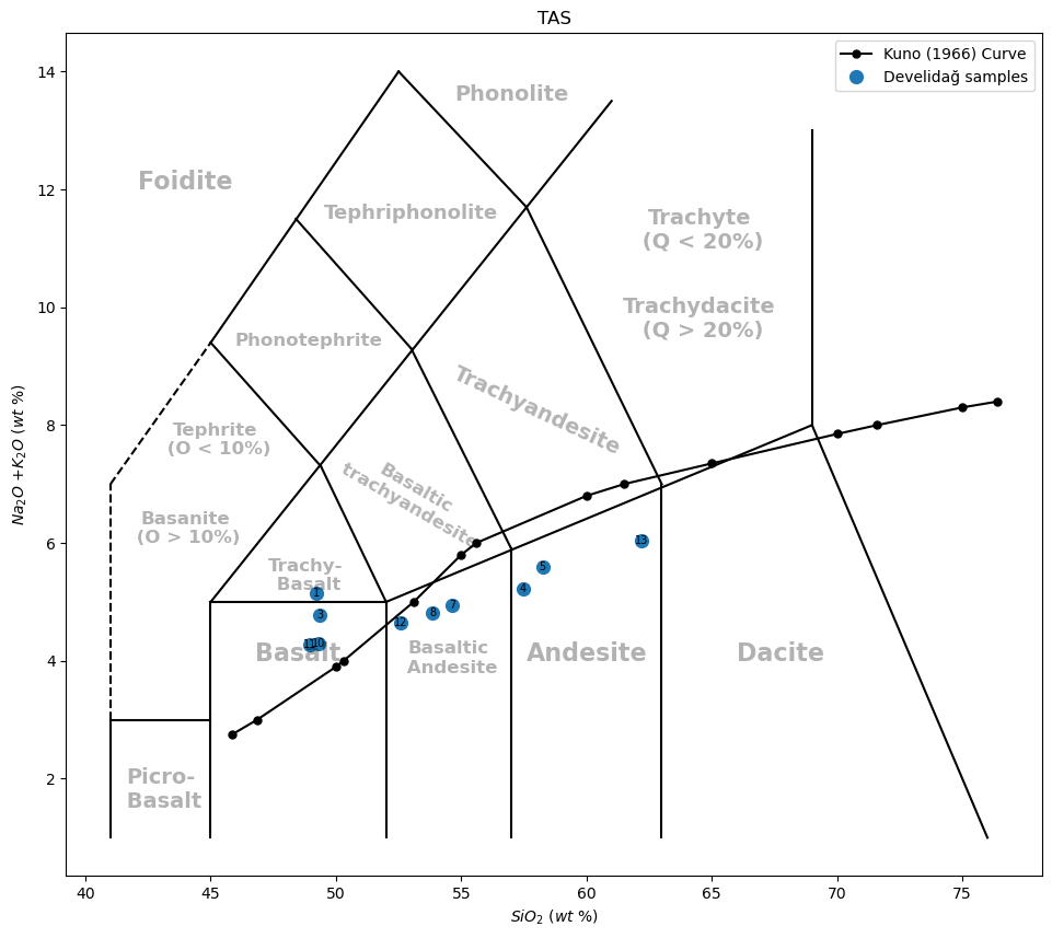

xx = np.linspace(45, 65, 1000)
p = np.polyfit(dataset.loc['SiO2'], dataset.loc['Na2O+K2O'], 2)
f = np.poly1d(p)
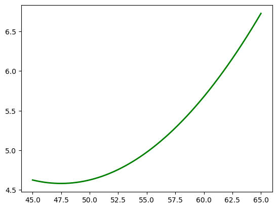
print(f)
plt.plot(xx, f(xx), "g-", lw=2)

          2
0.006996 x - 0.6645 x + 20.36

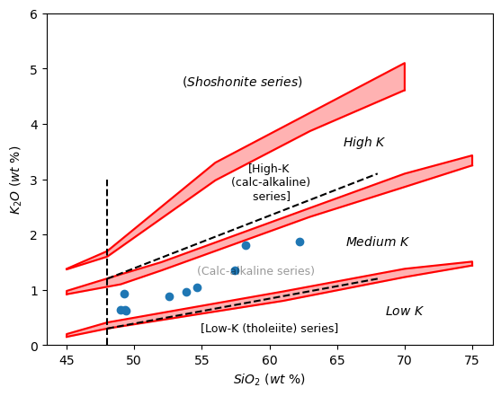
the subdivision of subalkalic rocks using the $K_{2}O \ vs \ SiO_{2}$ diagram¶

#shoshonite series
plt.plot((45.0, 48.0, 56.0, 63.0, 70.0, 70.0), (1.38, 1.7, 3.3, 4.2, 5.1, 4.61), "r-")
plt.plot((45.0, 48.0, 56.0, 63.0, 70.0), (1.37, 1.6, 2.98, 3.87, 4.61), "r-")
plt.fill_between((45.0, 48.0, 56.0, 63.0, 70.0), (1.38, 1.7, 3.3, 4.2, 5.1), (1.37, 1.6, 2.98, 3.87, 4.61), color="red", alpha=0.3)

#calc alkaline series
plt.plot((45.0, 45.0, 49.0, 52.0, 63.0, 70.0, 75.0, 75.0), (0.92, 0.98, 1.28, 1.5, 2.48, 3.1, 3.43, 3.25), "r-")
plt.plot((45.0, 49.0, 52.0, 63.0, 70.0, 75.0), (0.92, 1.1, 1.35, 2.32, 2.86, 3.25), "r-")
plt.fill_between((45.0, 49.0, 52.0, 63.0, 70.0, 75.0), (0.98, 1.28, 1.5, 2.48, 3.1, 3.43), (0.92, 1.1, 1.35, 2.32, 2.86, 3.25), color="red", alpha=0.3)

#low-K tholeiite series
plt.plot((45.0, 45.0, 48.0, 61.0, 70.0, 75.0, 75.0), (0.15, 0.2, 0.41, 0.97, 1.38, 1.51, 1.44), "r-")
plt.plot((45.0, 48.0, 61.0, 70.0, 75.0), (0.15, 0.3, 0.8, 1.23, 1.44), "r-")
plt.fill_between((45.0, 48.0, 61.0, 70.0, 75.0), (0.2, 0.41, 0.97, 1.38, 1.51), (0.15, 0.3, 0.8, 1.23, 1.44), color="red", alpha=0.3)


plt.plot((48.0, 68.0), (1.2, 3.1), "k--")
plt.plot((48.0, 68.0), (0.3, 1.2), "k--")
plt.xlabel(r'$SiO_{2} \ (wt \ \%)$'), plt.ylabel(r'$K_{2}O \ (wt \ \%)$')
plt.vlines(48, ymin=0, ymax=3, linestyles="--", colors="black")


plt.text(58, 4.7, r'$(Shoshonite \ series)$', ha="center")
plt.text(60, 2.65, "[High-K\n (calc-alkaline)\n series]", fontsize=9, ha="center")
plt.text(59, 1.28, "(Calc-alkaline series)", fontsize=9, ha="center")
plt.text(60, 0.25, "[Low-K (tholeiite) series]", fontsize=9, ha="center")
plt.text(67, 3.6, r'$High \ K$', ha="center")
plt.text(68, 1.8, r'$Medium \ K$', ha="center")
plt.text(70, 0.55, r'$Low \ K$', ha="center")

plt.ylim(0, 6)
plt.show()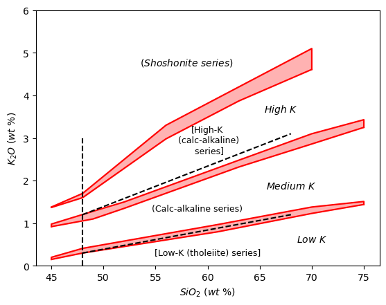

#shoshonite series
plt.plot((45.0, 48.0, 56.0, 63.0, 70.0, 70.0), (1.38, 1.7, 3.3, 4.2, 5.1, 4.61), "r-")
plt.plot((45.0, 48.0, 56.0, 63.0, 70.0), (1.37, 1.6, 2.98, 3.87, 4.61), "r-")
plt.fill_between((45.0, 48.0, 56.0, 63.0, 70.0), (1.38, 1.7, 3.3, 4.2, 5.1), (1.37, 1.6, 2.98, 3.87, 4.61), color="red", alpha=0.3)

#calc alkaline series
plt.plot((45.0, 45.0, 49.0, 52.0, 63.0, 70.0, 75.0, 75.0), (0.92, 0.98, 1.28, 1.5, 2.48, 3.1, 3.43, 3.25), "r-")
plt.plot((45.0, 49.0, 52.0, 63.0, 70.0, 75.0), (0.92, 1.1, 1.35, 2.32, 2.86, 3.25), "r-")
plt.fill_between((45.0, 49.0, 52.0, 63.0, 70.0, 75.0), (0.98, 1.28, 1.5, 2.48, 3.1, 3.43), (0.92, 1.1, 1.35, 2.32, 2.86, 3.25), color="red", alpha=0.3)

#low-K tholeiite series
plt.plot((45.0, 45.0, 48.0, 61.0, 70.0, 75.0, 75.0), (0.15, 0.2, 0.41, 0.97, 1.38, 1.51, 1.44), "r-")
plt.plot((45.0, 48.0, 61.0, 70.0, 75.0), (0.15, 0.3, 0.8, 1.23, 1.44), "r-")
plt.fill_between((45.0, 48.0, 61.0, 70.0, 75.0), (0.2, 0.41, 0.97, 1.38, 1.51), (0.15, 0.3, 0.8, 1.23, 1.44), color="red", alpha=0.3)


plt.plot((48.0, 68.0), (1.2, 3.1), "k--")
plt.plot((48.0, 68.0), (0.3, 1.2), "k--")
plt.xlabel(r'$SiO_{2} \ (wt \ \%)$'), plt.ylabel(r'$K_{2}O \ (wt \ \%)$')
plt.vlines(48, ymin=0, ymax=3, linestyles="--", colors="black")


plt.text(58, 4.7, r'$(Shoshonite \ series)$', ha="center")
plt.text(60, 2.65, "[High-K\n (calc-alkaline)\n series]", fontsize=9, ha="center")
plt.text(59, 1.28, "(Calc-alkaline series)", fontsize=9, ha="center", alpha=0.4)
plt.text(60, 0.25, "[Low-K (tholeiite) series]", fontsize=9, ha="center")
plt.text(67, 3.6, r'$High \ K$', ha="center")
plt.text(68, 1.8, r'$Medium \ K$', ha="center")
plt.text(70, 0.55, r'$Low \ K$', ha="center")

plt.plot(dataset.loc['SiO2'], dataset.loc['K2O'], "o")
plt.ylim(0, 6)
plt.show()

Develidağ TAS

Develidağ TAS¶

the subdivision of subalkalic rocks using the K2O vs SiO2K_{2}O \ vs \ SiO_{2}K2​O vs SiO2​ diagram¶

the subdivision of subalkalic rocks using the $K_{2}O \ vs \ SiO_{2}$ diagram¶