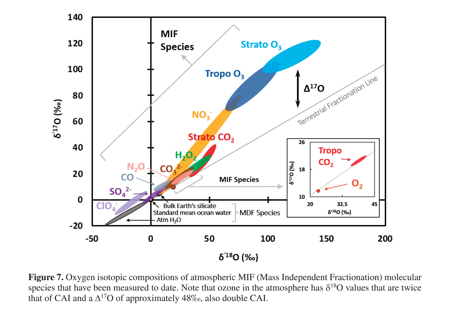
Isotope Geochemistry¶

Oxygen isotope notations¶

Oxygen has three stable isotopes:

$^{16}\mathrm{O}$
$^{17}\mathrm{O}$
$^{18}\mathrm{O}$

In stable isotope geochemistry, we usually compare the ratio of a heavy isotope to the most abundant isotope, $^{16}\mathrm{O}$ .

For oxygen isotopes:

R^{17} = \frac{^{17}\mathrm{O}}{^{16}\mathrm{O}}

(1)

R^{18} = \frac{^{18}\mathrm{O}}{^{16}\mathrm{O}}

(2)

Because absolute isotope ratios are very small and difficult to compare directly, isotope compositions are commonly reported relative to a reference material, such as VSMOW.

The delta notation is defined as:

\delta^{x}\mathrm{O} = \left( \frac{R^{x}_{\mathrm{sample}}}{R^{x}_{\mathrm{reference}}} -1 \right) \times 1000

(3)

where $x$ can be 17 or 18.

For example:

\delta^{18}\mathrm{O} = \left( \frac{ \left(^{18}\mathrm{O}/^{16}\mathrm{O}\right)_{\mathrm{sample}} }{ \left(^{18}\mathrm{O}/^{16}\mathrm{O}\right)_{\mathrm{reference}} } -1 \right) \times 1000

(4)

The result is reported in per mil, written as ‰.

A positive $\delta$ value means that the sample has a higher heavy-isotope/light-isotope ratio than the reference.

A negative $\delta$ value means that the sample has a lower heavy-isotope/light-isotope ratio than the reference.

Linearized delta notation: $\delta'$ notation¶

In triple oxygen isotope geochemistry, we often use the linearized form of delta notation.

This is called delta-prime notation:

\delta'^{x}\mathrm{O} = 1000 \ln \left( 1+ \frac{\delta^{x}\mathrm{O}}{1000} \right)

(5)

where $x$ can be 17 or 18.

Therefore:

\delta'^{17}\mathrm{O} = 1000 \ln \left( 1+ \frac{\delta^{17}\mathrm{O}}{1000} \right)

(6)

and

\delta'^{18}\mathrm{O} = 1000 \ln \left( 1+ \frac{\delta^{18}\mathrm{O}}{1000} \right)

(7)

For small isotope variations, $\delta$ and $\delta'$ are very similar.

However, $\delta'$ is mathematically useful because isotope fractionation becomes additive in logarithmic space.

Fractionation factor¶

The isotope fractionation factor between two phases, A and B, is defined as:

\alpha^{x}_{A-B} = \frac{R^{x}_{A}}{R^{x}_{B}}

(8)

where $R^{x}$ is the isotope ratio of isotope $x$ relative to $^{16}\mathrm{O}$ .

For oxygen isotopes:

\alpha^{18}_{A-B} = \frac{ \left(^{18}\mathrm{O}/^{16}\mathrm{O}\right)_A }{ \left(^{18}\mathrm{O}/^{16}\mathrm{O}\right)_B }

(9)

The fractionation factor can also be calculated from delta values:

\alpha^{x}_{A-B} = \frac{ 1+\delta^{x}O_A/1000 }{ 1+\delta^{x}O_B/1000 }

(10)

In isotope geochemistry, fractionation is often reported as:

1000 \ln \alpha^{x}_{A-B}

(11)

Using delta-prime notation:

1000 \ln \alpha^{x}_{A-B} = \delta'^{x}O_A - \delta'^{x}O_B

(12)

This is one reason why the logarithmic notation is useful.

Triple oxygen isotope relationship¶

In mass-dependent fractionation, $^{17}\mathrm{O}$ and $^{18}\mathrm{O}$ usually vary together.

Because $^{17}\mathrm{O}$ is intermediate in mass between $^{16}\mathrm{O}$ and $^{18}\mathrm{O}$ , the change in $\delta^{17}\mathrm{O}$ is approximately about half of the change in $\delta^{18}\mathrm{O}$ .

In linearized notation, this relationship is commonly written as:

\delta'^{17}\mathrm{O} = \lambda \delta'^{18}\mathrm{O} + \gamma

(13)

where:

$\lambda$ is the slope of the reference line
$\gamma$ is the intercept
$\delta'^{17}\mathrm{O}$ and $\delta'^{18}\mathrm{O}$ are the linearized isotope values

A commonly used simplified form is:

\delta'^{17}\mathrm{O} = \lambda \delta'^{18}\mathrm{O}

(14)

with, for example:

\lambda = 0.528

(15)

This line represents the expected mass-dependent relationship between $^{17}\mathrm{O}$ and $^{18}\mathrm{O}$ .

Capital delta (Cap Delta) notation: $\Delta'^{17}\mathrm{O}$ ¶

The parameter $\Delta'^{17}\mathrm{O}$ describes the deviation of a sample from a chosen mass-dependent reference line.

It is commonly defined as:

\Delta'^{17}\mathrm{O} = \delta'^{17}\mathrm{O} - \lambda \delta'^{18}\mathrm{O}

(16)

where $\lambda$ is the chosen reference slope.

If the reference line includes an intercept, the equation becomes:

\Delta'^{17}\mathrm{O} = \delta'^{17}\mathrm{O} - \left( \lambda \delta'^{18}\mathrm{O} + \gamma \right)

(17)

If $\Delta'^{17}\mathrm{O} = 0$ , the sample lies exactly on the chosen reference line.

If $\Delta'^{17}\mathrm{O} > 0$ , the sample lies above the reference line.

If $\Delta'^{17}\mathrm{O} < 0$ , the sample lies below the reference line.

Because $\Delta'^{17}\mathrm{O}$ values are usually very small, they are often reported in per meg:

\Delta'^{17}\mathrm{O}_{\mathrm{per\ meg}} = 1000 \left[ \delta'^{17}\mathrm{O} - \lambda \delta'^{18}\mathrm{O} \right]

(18)

Here, $\delta'^{17}\mathrm{O}$ and $\delta'^{18}\mathrm{O}$ are in per mil, while $\Delta'^{17}\mathrm{O}_{\mathrm{per\ meg}}$ is in per meg.

$\theta$ and $\lambda$ ¶

In triple oxygen isotope geochemistry, both $\theta$ and $\lambda$ describe slopes in oxygen isotope space, but they are often used differently.

The exponent $\theta$ is commonly used for a specific fractionation process between two phases:

\theta_{A-B} = \frac{ \ln \alpha^{17}_{A-B} }{ \ln \alpha^{18}_{A-B} }

(19)

For example, $\theta$ may describe equilibrium fractionation between quartz and water, or another specific mineral-fluid pair.

The parameter $\lambda$ is commonly used for a reference line or empirical relationship in isotope space:

\delta'^{17}\mathrm{O} = \lambda \delta'^{18}\mathrm{O} + \gamma

(20)

In simple terms:

$\theta$ describes the slope of a specific fractionation process.
$\lambda$ describes the slope of a chosen reference line.

Because $\Delta'^{17}\mathrm{O}$ depends on the chosen reference slope, the value of $\lambda$ should always be reported.

import pandas as pd
import numpy as np
import matplotlib.pyplot as plt

c:\Users\altar\anaconda3\Lib\site-packages\pandas\core\computation\expressions.py:23: UserWarning: Pandas requires version '2.10.2' or newer of 'numexpr' (version '2.10.1' currently installed).
  from pandas.core.computation.check import NUMEXPR_INSTALLED

data = pd.read_excel('./data/Data_Altar_140225.xlsx')
data = data.iloc[:13]

Develidag = pd.read_excel('./data/Develidag.xlsx')
Develidag

SCOL_dataset = pd.read_excel('./data/SCOL_data.xlsx')

creating a new pandas dataframe with the given corrected values

corrected_dataset = pd.DataFrame()
corrected_dataset['Sample'] = Develidag['SampleName']
corrected_dataset['Sample Type'] = Develidag['SampleType']
corrected_dataset['d17O'], corrected_dataset['d18O'] = Develidag['cd_d17O'], Develidag['cd_d18O']
corrected_dataset['dp17O'], corrected_dataset['dp18O'] = Develidag['dp17O'], Develidag['dp18O']
corrected_dataset['D17O'] = Develidag['cd_D17O']
corrected_dataset

SCOL_data = pd.DataFrame()
SCOL_data['Sample'] = SCOL_dataset['SampleName']
SCOL_data['Sample Type'] = SCOL_dataset['SampleType']
SCOL_data['d17O'], SCOL_data['d18O'] = SCOL_dataset['cd_d17O'], SCOL_dataset['cd_d18O']
SCOL_data['dp17O'], SCOL_data['dp18O'] = SCOL_dataset['dp17O'], SCOL_dataset['dp18O']
SCOL_data['D17O'] = SCOL_dataset['cd_D17O']
SCOL_data

np.mean(SCOL_data['d17O']), np.mean(SCOL_data['d18O']), np.mean(SCOL_data['D17O'])

(np.float64(2.7037898284644477), np.float64(5.226), np.float64(-52.0))

olivine_data = corrected_dataset[corrected_dataset['Sample Type'] == 'Olivine'].reset_index(drop=True)
opx_data = corrected_dataset[corrected_dataset['Sample Type'] == 'Orthopyroxene'].reset_index(drop=True)
cpx_data = corrected_dataset[corrected_dataset['Sample Type'] == 'Clinopyroxene'].reset_index(drop=True)
bulk_data = corrected_dataset[corrected_dataset['Sample Type'] == 'Mafic volcanics '].reset_index(drop=True)

bulk_data

triple oxygen isotope plots

plt.plot(olivine_data['d18O'], olivine_data['D17O']/1000, "yo", label='Olivine')
plt.plot(cpx_data['d18O'], cpx_data['D17O']/1000, "o", color='darkgreen', label='Clinopyroxene')
plt.plot(opx_data['d18O'], opx_data['D17O']/1000, "o", color='brown', label='Orthopyroxene')
plt.plot(SCOL_data['d18O'], SCOL_data['D17O']/1000, "o", color='lightgreen', label='San Carlos Olivine')
plt.plot(bulk_data['d18O'], bulk_data['D17O']/1000, "ko", label='whole rock')
plt.xlabel(r'$\delta^{18}O\ (‰ \ VSMOW)$'), plt.ylabel(r"$\Delta^{'17}O_{0.528}\ (‰ \ VSMOW)$")
plt.title('Develidağ Triple Plot')
plt.legend()
plt.show()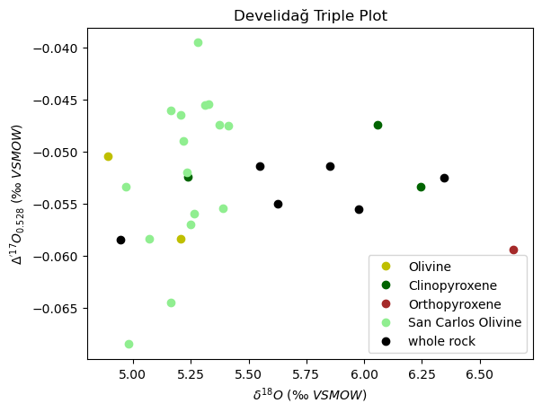

x = pd.concat([corrected_dataset, SCOL_data], ignore_index=True)['dp18O']
y = pd.concat([corrected_dataset, SCOL_data], ignore_index=True)['dp17O']
m, b = np.polyfit(x, y, 1)
def f(x):
    return m*x + b

xx = np.linspace(x.min(), x.max(), 200)

print(m)

0.5284319177388419

np.polyfit(corrected_dataset['dp18O'], corrected_dataset['dp17O'], 1)

array([ 0.5280339 , -0.05400147])

np.polyfit(bulk_data['dp18O'], bulk_data['dp17O'], 1)

array([ 0.53164102, -0.0747995 ])

plt.plot(xx, f(xx), "r--", label=f'fitted line (slope={m:.3f})')
plt.plot(olivine_data['dp18O'], olivine_data['dp17O'], "yo", label='Olivine')
plt.plot(cpx_data['dp18O'], cpx_data['dp17O'], "o", color='darkgreen', label='Clinopyroxene')
plt.plot(opx_data['dp18O'], opx_data['dp17O'], "o", color='brown', label='Orthopyroxene')
plt.plot(SCOL_data['dp18O'], SCOL_data['dp17O'], "o", color='lightgreen', label='San Carlos Olivine')
plt.plot(bulk_data['dp18O'], bulk_data['dp17O'], "ko", label='whole rock')
plt.xlabel(r'$\delta^{\prime 18}O\ (\perthousand \ VSMOW)$'), plt.ylabel(r"$\delta^{\prime 17}O\ (\perthousand \ VSMOW)$")
plt.title('Develidağ Triple Plot')
plt.legend()
plt.show()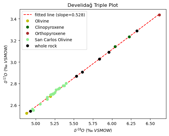

values from Pack & Herwartz 2014

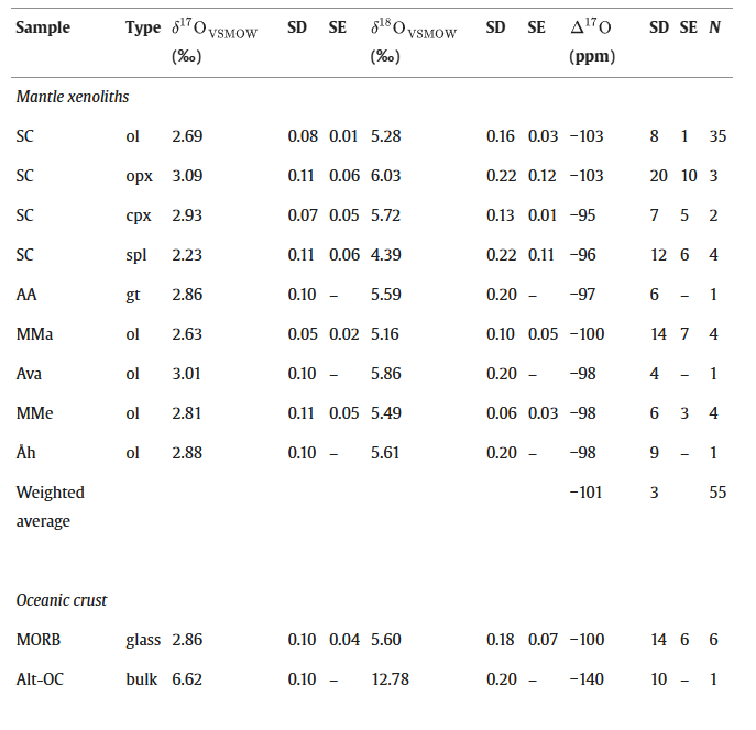
plt.plot(5.28, -103/1000, "s", label='San Carlos Olivine')
plt.plot(6.03, -103/1000, "s", color='brown', label='San Carlos opx')
plt.plot(5.72, -95/1000, "s", color='darkgreen', label='San Carlos cpx')
plt.plot(5.60, -100/1000, "s", color='black', label='MORB')
plt.xlabel(r'$\delta^{18}O\ (‰)$'), plt.ylabel(r"$\Delta^{'17}O\ (‰)$")
plt.title('Mantle values (from Pack & Herwartz 2014)')
plt.legend()
plt.show()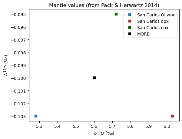

plt.plot(olivine_data['d18O'], olivine_data['D17O']/1000, "yo", label='Olivine')
plt.plot(cpx_data['d18O'], cpx_data['D17O']/1000, "o", color='darkgreen', label='Clinopyroxene')
plt.plot(opx_data['d18O'], opx_data['D17O']/1000, "o", color='brown', label='Orthopyroxene')
plt.plot(SCOL_data['d18O'], SCOL_data['D17O']/1000, "o", color='lightgreen', label='San Carlos Olivine')
plt.plot(bulk_data['d18O'], bulk_data['D17O']/1000, "ko", label='whole rock')
plt.plot(5.28, -103/1000, "s", color='lightgreen', label='San Carlos Olivine')
plt.plot(6.03, -103/1000, "s", color='brown', label='San Carlos opx')
plt.plot(5.72, -95/1000, "s", color='darkgreen', label='San Carlos cpx')
plt.plot(5.60, -100/1000, "s", color='black', label='MORB')
plt.xlabel(r'$\delta^{18}O\ (‰)$'), plt.ylabel(r"$\Delta^{'17}O\ (‰)$")
plt.title('Develidağ vs Mantle values')
plt.legend()
plt.show()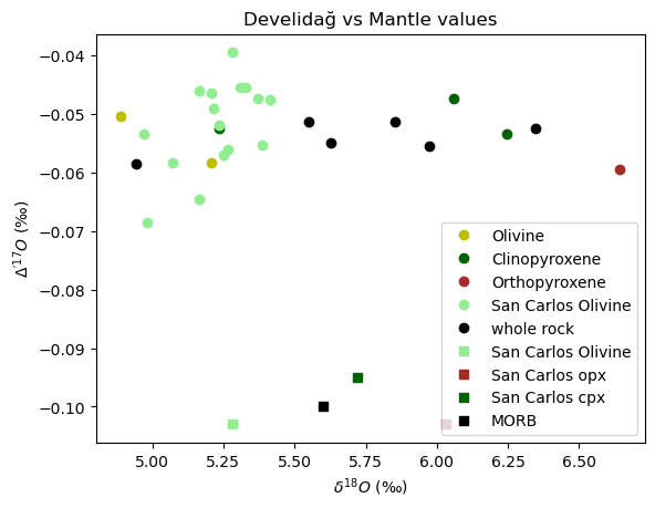

plt.plot(SCOL_data['d18O'], SCOL_data['D17O']/1000, "o", color='lightgreen', label='San Carlos Olivine')
plt.plot(olivine_data['d18O'], olivine_data['D17O']/1000, "yo", label='Olivine')
plt.plot(cpx_data['d18O'], cpx_data['D17O']/1000, "o", color='darkgreen', label='Clinopyroxene')
plt.plot(opx_data['d18O'], opx_data['D17O']/1000, "o", color='brown', label='Orthopyroxene')
plt.plot(bulk_data['d18O'], bulk_data['D17O']/1000, "ko", label='whole rock')
plt.xlabel(r'$\delta^{18}O\ (‰)$'), plt.ylabel(r"$\Delta^{'17}O\ (‰)$")
plt.title('Develidağ Triple Plot')
plt.legend()
plt.show()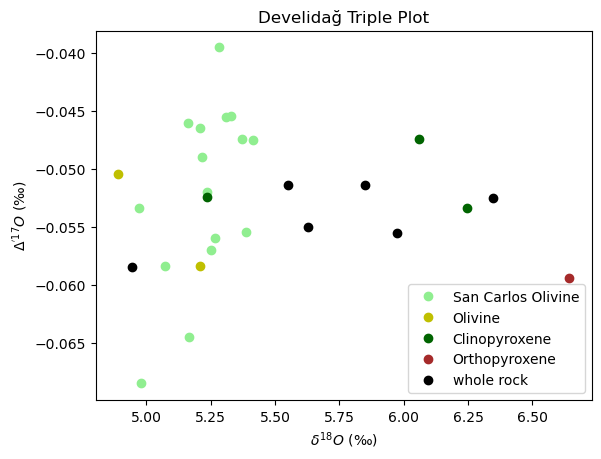

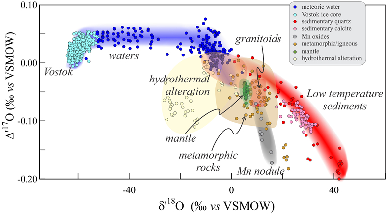
implementation of stable isotopes vs. radiogenic isotopes; plots etc.

bulk_data

radiogenic_data = pd.read_excel('./D2004_radiogenic.xlsx', index_col=0)
radiogenic_data

plt.plot(radiogenic_data['D2004-3']['87Sr/86Sr'], bulk_data['d18O'][2], "o", color='black')
plt.plot(radiogenic_data['D2004-11']['87Sr/86Sr'], bulk_data['d18O'][1], "o", color='black')
plt.xlabel(r'$^{87}Sr/^{86}Sr$'), plt.ylabel(r'$\delta^{18}O$')
plt.title('d18O vs Sr')
plt.show()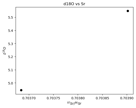

plt.plot(0.703, 6.0, "ko") #A
plt.plot(0.710, 12.0, "ko") #B
plt.xlabel(r'$^{87}Sr/^{86}Sr$'), plt.ylabel(r'$\delta^{18}O \ (\perthousand)$')
plt.title('d18O vs Sr')
plt.show()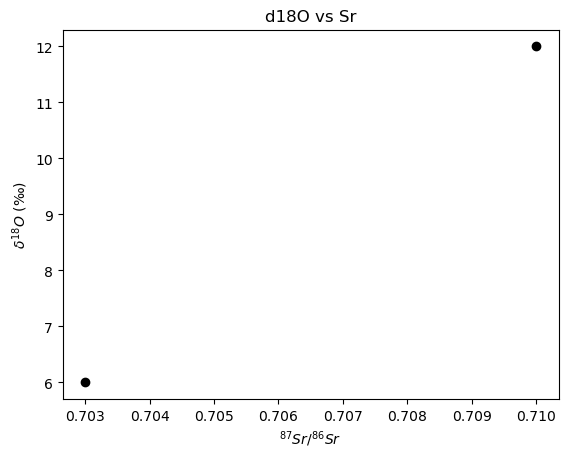

Hyperbolic Mixing Equation¶

The isotopic ratio of the mixture is given by:

\left( \frac{^{87}\text{Sr}}{^{86}\text{Sr}} \right)_{\text{mix}} = \frac{[\text{Sr}]_A \cdot \left( \frac{^{87}\text{Sr}}{^{86}\text{Sr}} \right)_A \cdot (1 - x) + [\text{Sr}]_B \cdot \left( \frac{^{87}\text{Sr}}{^{86}\text{Sr}} \right)_B \cdot x \cdot r}{[\text{Sr}]_A \cdot (1 - x) + [\text{Sr}]_B \cdot x \cdot r}

(21)

Where:

$[\text{Sr}]_A$ , $[\text{Sr}]_B$ = Sr concentrations in end-members A (mantle) and B (crust)
$r = \frac{[\text{Sr}]_B}{[\text{Sr}]_A}$ = concentration ratio (5:1, 1:10, etc.)
$x$ = mixing fraction (0 to 1)

\delta^{18}\text{O}_{\text{mix}} = \delta^{18}\text{O}_A (1 - x) + \delta^{18}\text{O}_B \cdot x \ \ \text{(linear mixing for oxygen)}

(22)

# Define end-members (A = mantle, B = crust)
A = np.array([0.703, 6.0])   # Low 87Sr/86Sr, low δ18O (mantle)
B = np.array([0.710, 12.0])  # High 87Sr/86Sr, high δ18O (crust)

# Mixing parameter (fraction of contaminant, x)
x = np.linspace(0, 1, 100)

# Sr concentration ratios (Sr_B/Sr_A) to test
ratios = [0.2, 0.5, 1, 2, 10]  # 5:1, 2:1, 1:1, 1:2, 1:10

plt.figure(figsize=(8,6))

Sr_array = []
O_array = []

for i, ratio in enumerate(ratios):
    # Hyperbolic mixing for Sr isotopes
    Sr_mix = (A[0] * (1 - x) + B[0] * x * ratio) / (1 - x + x * ratio)
    Sr_array.append(Sr_mix)
    # Linear mixing for O isotopes (no fractionation)
    O_mix = A[1] * (1 - x) + B[1] * x
    O_array.append(O_mix)
    
    plt.plot(Sr_mix, O_mix, color="black", lw=2)


plt.fill_betweenx(O_array[0], Sr_array[1], Sr_array[0], color="black", alpha=0.15)
plt.fill_betweenx(O_array[4], Sr_array[4], Sr_array[3], color="black", alpha=0.15)
plt.text(A[0]-0.00025, A[1]-0.15, "A", fontsize=12, weight="bold")
plt.text(B[0]+0.00015, B[1]+0.02, "B", fontsize=12, weight="bold")
plt.text(0.7073, 7.1, "Source Contamination", fontsize=12, ha="center", rotation=20)
plt.text(0.7053, 8.72, "Crustal Contamination", fontsize=12, ha="center", rotation=35)
plt.text(0.7049, 10, "5:1", fontsize=12, ha="center", rotation=35)
plt.text(0.7055, 9.15, "2:1", fontsize=12, ha="center", rotation=35)
plt.text(0.7065, 9, "1:1", fontsize=12, ha="center", rotation=35)
plt.text(0.7070, 8.44, "1:2", fontsize=12, ha="center", rotation=35)
plt.text(0.7080, 7.2, "1:5", fontsize=12, ha="center", rotation=32)
plt.plot(A[0], A[1], "ko", markersize=8, label="Mantle (A)")
plt.plot(B[0], B[1], "ko", markersize=8, label="Crust (B)")
plt.plot(radiogenic_data['D2004-3']['87Sr/86Sr'], bulk_data['d18O'][2], "s", color='black', label="D2004, 3 & 11")
plt.plot(radiogenic_data['D2004-11']['87Sr/86Sr'], bulk_data['d18O'][1], "s", color='black')
plt.xlabel(r'$^{87}Sr/^{86}Sr$', fontsize=12)
plt.ylabel(r'$\delta^{18}O \ (\perthousand)$', fontsize=12)
plt.title("Hypothetical mixing diagram (James, 1981)", fontsize=14)
plt.legend()
plt.show()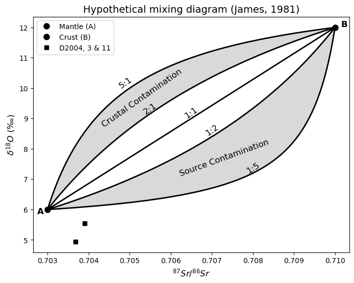

er_data = [
    ("ER 1",     0.705084, 6.89),
    ("ER 2",     np.nan,   np.nan),
    ("ER 3",     0.704537, 6.82),
    ("ER4",      np.nan,   np.nan),
    ("ER5",      np.nan,   np.nan),
    ("ER9",      0.704511, 6.51),
    ("ER10",     0.704587, 6.46),
    ("ER11",     0.704710, 6.37),
    ("ER13",     0.703609, 6.05),
    ("ER16",     np.nan,   np.nan),
    ("ER17",     0.704534, 6.79),
    ("ER20",     0.704697, 6.80),
    ("ER22",     0.704769, 6.47),
    ("ER25",     np.nan,   np.nan),
    ("ER26",     0.704875, 6.51),
    ("ER27(1)",  0.704796, 6.15),
    ("ER27(2)",  0.704817, 6.15),
    ("ER29",     0.704876, 6.63),
    ("ER30",     0.704509, 7.12),
    ("ER32",     0.704557, 6.00)
]

# Create DataFrame
Erciyes_data = pd.DataFrame(er_data, columns=["Sample", "87Sr/86Sr", "d18O_WR"])
Erciyes_data

sw_cap = {
    'Group': [
        "HS", "OZ", "OZ", "OZ", "OZ",
        "HS", "HS", "HS", "HS", "OZ",
        "OZ", "HS", "K", "K", "K"
    ],
    '87Sr/86Sr': [
        0.704952, 0.704333, 0.704319, 0.704711, 0.704472,
        0.704636, 0.704729, 0.704908, 0.704625, 0.704153,
        0.704542, 0.704976, 0.705320, 0.705188, 0.705502
    ],
    'd18O_WR': [
        6.79, 6.57, 6.58, 6.61, 6.38,
        6.73, 6.62, 6.63, 6.92, 5.88,
        7.27, 6.68, 6.75, 6.59, 6.31
    ]
}

# Create full DataFrame
df_sw_cap = pd.DataFrame(sw_cap)

# Split into separate group DataFrames
df_HS = df_sw_cap[df_sw_cap['Group'] == 'HS'].reset_index(drop=True)
df_OZ = df_sw_cap[df_sw_cap['Group'] == 'OZ'].reset_index(drop=True)
df_K  = df_sw_cap[df_sw_cap['Group'] == 'K'].reset_index(drop=True)

df_HS

d18O vs 87Sr/86Sr - Mixing Diagram¶

# Define end-members (A = mantle, B = crust)
A = np.array([0.703, 6.0])   # Low 87Sr/86Sr, low δ18O (mantle)
B = np.array([0.710, 12.0])  # High 87Sr/86Sr, high δ18O (crust)

# Mixing parameter (fraction of contaminant, x)
x = np.linspace(0, 1, 100)

# Sr concentration ratios (Sr_B/Sr_A) to test
ratios = [0.2, 0.5, 1, 2, 10]  # 5:1, 2:1, 1:1, 1:2, 1:10

plt.figure(figsize=(8,6))

Sr_array = []
O_array = []

for i, ratio in enumerate(ratios):
    # Hyperbolic mixing for Sr isotopes
    Sr_mix = (A[0] * (1 - x) + B[0] * x * ratio) / (1 - x + x * ratio)
    Sr_array.append(Sr_mix)
    # Linear mixing for O isotopes (no fractionation)
    O_mix = A[1] * (1 - x) + B[1] * x
    O_array.append(O_mix)
    
    plt.plot(Sr_mix, O_mix, color="black", lw=2)


plt.fill_betweenx(O_array[0], Sr_array[1], Sr_array[0], color="black", alpha=0.15)
plt.fill_betweenx(O_array[4], Sr_array[4], Sr_array[3], color="black", alpha=0.15)
plt.text(A[0]-0.00025, A[1]-0.15, "A", fontsize=12, weight="bold")
plt.text(B[0]+0.00015, B[1]+0.02, "B", fontsize=12, weight="bold")
plt.text(0.7073, 7.1, "Source Contamination", fontsize=12, ha="center", rotation=20)
plt.text(0.7053, 8.72, "Crustal Contamination", fontsize=12, ha="center", rotation=35)
plt.text(0.7049, 10, "5:1", fontsize=12, ha="center", rotation=35)
plt.text(0.7055, 9.15, "2:1", fontsize=12, ha="center", rotation=35)
plt.text(0.7065, 9, "1:1", fontsize=12, ha="center", rotation=35)
plt.text(0.7070, 8.44, "1:2", fontsize=12, ha="center", rotation=35)
plt.text(0.7080, 7.2, "1:5", fontsize=12, ha="center", rotation=32)
plt.plot(A[0], A[1], "ko", markersize=8, label="Mantle (A)")
plt.plot(B[0], B[1], "ko", markersize=8, label="Crust (B)")
plt.plot(radiogenic_data['D2004-3']['87Sr/86Sr'], bulk_data['d18O'][1], "s", color='black', label="D2004, 3&11")
plt.plot(radiogenic_data['D2004-11']['87Sr/86Sr'], bulk_data['d18O'][0], "s", color='black')
plt.plot(Erciyes_data['87Sr/86Sr'], Erciyes_data['d18O_WR'], "s", color='blue', label="Erciyes")
plt.plot(df_HS['87Sr/86Sr'], df_HS['d18O_WR'], "s", color='green', label='Hasandağ')
plt.plot(df_K['87Sr/86Sr'], df_K['d18O_WR'], "s", color='red', label='Karapınar')
plt.plot(df_OZ['87Sr/86Sr'], df_OZ['d18O_WR'], "s", color='yellow', label='Obruk-Zengen')
plt.xlabel(r'$^{87}Sr/^{86}Sr$', fontsize=12)
plt.ylabel(r'$\delta^{18}O \ (\perthousand)$', fontsize=12)
plt.title("Hypothetical mixing diagram (James, 1981)", fontsize=14)
plt.legend()
plt.show()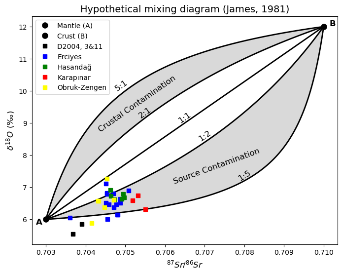

# Define end-members (A = mantle, B = crust)
A = np.array([0.703, 6.0])   # Low 87Sr/86Sr, low δ18O (mantle)
B = np.array([0.710, 12.0])  # High 87Sr/86Sr, high δ18O (crust)

# Mixing parameter (fraction of contaminant, x)
x = np.linspace(0, 1, 100)

# Sr concentration ratios (Sr_B/Sr_A) to test
ratios = [0.2, 0.5, 1, 2, 10]  # 5:1, 2:1, 1:1, 1:2, 1:10

plt.figure(figsize=(8,6))

Sr_array = []
O_array = []

for i, ratio in enumerate(ratios):
    # Hyperbolic mixing for Sr isotopes
    Sr_mix = (A[0] * (1 - x) + B[0] * x * ratio) / (1 - x + x * ratio)
    Sr_array.append(Sr_mix)
    # Linear mixing for O isotopes (no fractionation)
    O_mix = A[1] * (1 - x) + B[1] * x
    O_array.append(O_mix)
    
    plt.plot(Sr_mix, O_mix, color="black", lw=2)


plt.fill_betweenx(O_array[0], Sr_array[1], Sr_array[0], color="black", alpha=0.15)
plt.fill_betweenx(O_array[4], Sr_array[4], Sr_array[3], color="black", alpha=0.15)
plt.text(A[0]-0.00025, A[1]-0.15, "A", fontsize=12, weight="bold")
plt.text(B[0]+0.00015, B[1]+0.02, "B", fontsize=12, weight="bold")
plt.text(0.7073, 7.1, "Source Contamination", fontsize=12, ha="center", rotation=20)
plt.text(0.7053, 8.72, "Crustal Contamination", fontsize=12, ha="center", rotation=35)
plt.text(0.7049, 10, "5:1", fontsize=12, ha="center", rotation=35)
plt.text(0.7055, 9.15, "2:1", fontsize=12, ha="center", rotation=35)
plt.text(0.7065, 9, "1:1", fontsize=12, ha="center", rotation=35)
plt.text(0.7070, 8.44, "1:2", fontsize=12, ha="center", rotation=35)
plt.text(0.7080, 7.2, "1:5", fontsize=12, ha="center", rotation=32)
plt.plot(A[0], A[1], "ko", markersize=8, label="Mantle (A)")
plt.plot(B[0], B[1], "ko", markersize=8, label="Crust (B)")
plt.plot(radiogenic_data['D2004-3']['87Sr/86Sr'], bulk_data['d18O'][1], "s", color='black', label="Develidağ") #DEVELİDAĞ
plt.plot(radiogenic_data['D2004-11']['87Sr/86Sr'], bulk_data['d18O'][0], "s", color='black')
plt.plot(radiogenic_data['D2004-5']['87Sr/86Sr'], bulk_data['d18O'][4], "s", color='black')
plt.plot(radiogenic_data['D2004-7']['87Sr/86Sr'], bulk_data['d18O'][5], "s", color='black')
plt.plot(radiogenic_data['D2004-8']['87Sr/86Sr'], bulk_data['d18O'][3], "s", color='black')
plt.plot(radiogenic_data['D2004-12']['87Sr/86Sr'], bulk_data['d18O'][2], "s", color='black')
plt.plot(Erciyes_data['87Sr/86Sr'], Erciyes_data['d18O_WR'], "s", color='blue', label="Erciyes")
plt.plot(df_HS['87Sr/86Sr'], df_HS['d18O_WR'], "s", color='green', label='Hasandağ')
plt.plot(df_K['87Sr/86Sr'], df_K['d18O_WR'], "s", color='red', label='Karapınar')
plt.plot(df_OZ['87Sr/86Sr'], df_OZ['d18O_WR'], "s", color='yellow', label='Obruk-Zengen')
plt.xlabel(r'$^{87}Sr/^{86}Sr$', fontsize=12)
plt.ylabel(r'$\delta^{18}O \ (\perthousand)$', fontsize=12)
plt.title("Hypothetical mixing diagram (James, 1981)", fontsize=14)
plt.legend()
plt.show()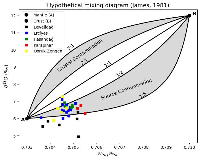

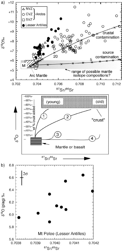
D2004-3 ve D2004-11, manto kökenli ve yay ile ilişkili

Davidson, J. P., et al. (2005).

plt.plot(radiogenic_data['D2004-3']['143Nd/144Nd'], bulk_data['d18O'][2], "o", color='black')
plt.plot(radiogenic_data['D2004-11']['143Nd/144Nd'], bulk_data['d18O'][1], "o", color='black')
plt.xlabel(r'$^{143}Nd/^{144}Nd$'), plt.ylabel(r'$\delta^{18}O$')
plt.title('d18O vs Nd')
plt.xlim(0.4,0.6)
plt.show()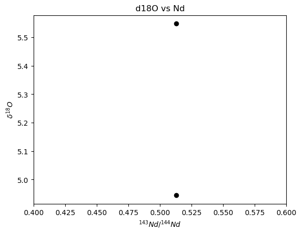

εNd hesabı¶

def epsilon_nd(nd_143_144_sample):
    # CHUR reference value for 143Nd/144Nd
    nd_143_144_chur = 0.512638

    # εNd
    epsilon_nd = ((nd_143_144_sample / nd_143_144_chur) - 1) * 10**4

    return epsilon_nd

plt.plot(epsilon_nd(radiogenic_data['D2004-3']['143Nd/144Nd']), bulk_data['d18O'][2], "o", color='black')
plt.plot(epsilon_nd(radiogenic_data['D2004-11']['143Nd/144Nd']), bulk_data['d18O'][1], "o", color='black')
plt.xlabel(r'eNd'), plt.ylabel(r'$\delta^{18}O$')
plt.title('d18O vs eNd')
plt.show()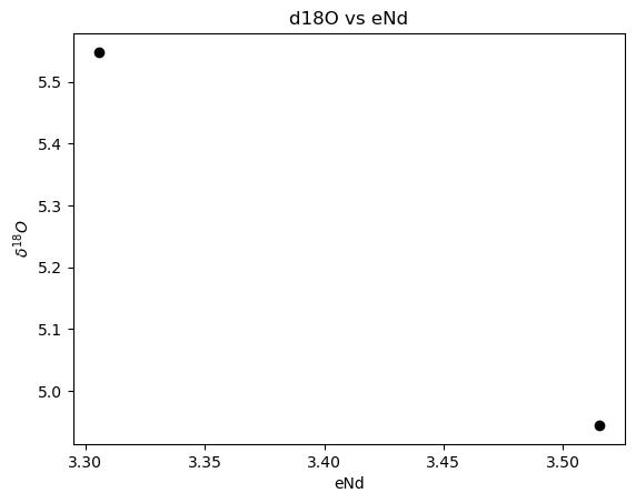

pozitif eNd değerleri manto kökenini gösterir.

major_trace_element = pd.read_excel("../D2004_1.xlsx", index_col=0)
major_trace_element

---------------------------------------------------------------------------
FileNotFoundError                         Traceback (most recent call last)
Cell In[78], line 1
----> 1 major_trace_element = pd.read_excel("../D2004_1.xlsx", index_col=0)
      2 major_trace_element

File c:\Users\altar\anaconda3\Lib\site-packages\pandas\io\excel\_base.py:495, in read_excel(io, sheet_name, header, names, index_col, usecols, dtype, engine, converters, true_values, false_values, skiprows, nrows, na_values, keep_default_na, na_filter, verbose, parse_dates, date_parser, date_format, thousands, decimal, comment, skipfooter, storage_options, dtype_backend, engine_kwargs)
    493 if not isinstance(io, ExcelFile):
    494     should_close = True
--> 495     io = ExcelFile(
    496         io,
    497         storage_options=storage_options,
    498         engine=engine,
    499         engine_kwargs=engine_kwargs,
    500     )
    501 elif engine and engine != io.engine:
    502     raise ValueError(
    503         "Engine should not be specified when passing "
    504         "an ExcelFile - ExcelFile already has the engine set"
    505     )

File c:\Users\altar\anaconda3\Lib\site-packages\pandas\io\excel\_base.py:1550, in ExcelFile.__init__(self, path_or_buffer, engine, storage_options, engine_kwargs)
   1548     ext = "xls"
   1549 else:
-> 1550     ext = inspect_excel_format(
   1551         content_or_path=path_or_buffer, storage_options=storage_options
   1552     )
   1553     if ext is None:
   1554         raise ValueError(
   1555             "Excel file format cannot be determined, you must specify "
   1556             "an engine manually."
   1557         )

File c:\Users\altar\anaconda3\Lib\site-packages\pandas\io\excel\_base.py:1402, in inspect_excel_format(content_or_path, storage_options)
   1399 if isinstance(content_or_path, bytes):
   1400     content_or_path = BytesIO(content_or_path)
-> 1402 with get_handle(
   1403     content_or_path, "rb", storage_options=storage_options, is_text=False
   1404 ) as handle:
   1405     stream = handle.handle
   1406     stream.seek(0)

File c:\Users\altar\anaconda3\Lib\site-packages\pandas\io\common.py:882, in get_handle(path_or_buf, mode, encoding, compression, memory_map, is_text, errors, storage_options)
    873         handle = open(
    874             handle,
    875             ioargs.mode,
   (...)
    878             newline="",
    879         )
    880     else:
    881         # Binary mode
--> 882         handle = open(handle, ioargs.mode)
    883     handles.append(handle)
    885 # Convert BytesIO or file objects passed with an encoding

FileNotFoundError: [Errno 2] No such file or directory: '../D2004_1.xlsx'

SiO2 = major_trace_element.loc["SiO2"]
Al2O3 = major_trace_element.loc["Al2O3"]
Na2O = major_trace_element.loc["Na2O"]
K2O = major_trace_element.loc["K2O"]
MgO = major_trace_element.loc["MgO"]
CaO = major_trace_element.loc["CaO"]
TiO2 = major_trace_element.loc["TiO2"]
P2O5 = major_trace_element.loc["P2O5 "]
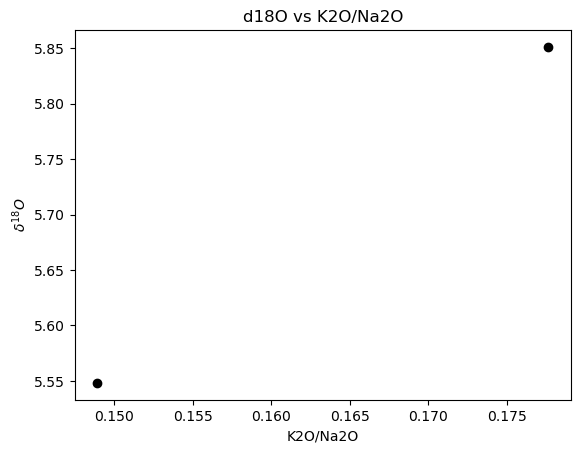
FeO = major_trace_element.iloc[8]

(K2O/Na2O).loc['D2004-3']

0.1489213045360527

plt.plot((K2O/Na2O).loc['D2004-3'], bulk_data['d18O'][2], "o", color='black')
plt.plot((K2O/Na2O).loc['D2004-11'], bulk_data['d18O'][1], "o", color='black')
plt.xlabel('K2O/Na2O'), plt.ylabel(r'$\delta^{18}O$')
plt.title('d18O vs K2O/Na2O')
plt.show()

Isotope Geochemistry